Learn how to build a shiny app for the visualization of clustering results. The app helps to better identify patient data samples, e.g. during a clinical study.
The story behind this app comes from a real application inside departments evaluating clinical studies in diagnostics.
Due to fast recruiting for clinical studies the patient cohorts seemed to be inhomogenic. Therefore a researcher and a clinical study statistician wanted to find out, by which parameter they can find patients, that do not seem to fit their desired class. Maybe there was a mistake in the labeling of a patient’s disease status? Maybe one measurement or two measurements can be used to easily find such patients?
The example data used here is real data from a 1990’s study, known as the biopsy data set, also hosted on UCI ML data repository. The app that should be build inside this tutorial is preliminary and was especially build for the tutorial. Pieces of it were applied in real world biostatistical applications.
if you have all the packages installed you will have one file to work on. This file is app.R. This app.R allows you to build a shiny application.
This file we will use to insert the right visualizations and the right table for the researcher to fullfil the task named above. To check what the app will finally look like you can already perform runApp() inside the console and your browser will open the app.
The app already contains:
A sideBarPanel that has all the inputs we need
Slider for the # of patients
Slider for the # of desired clusters/groups
Empty input to choose measurements — shall be done by you
Dropdown field for the clustering method
A server function that will provide
The empty input to choose measurments
A Heatmap to see the outcome of clustering
A Phylogenetic tree plot to see the outcome of clustering
A table to see the outcome of the clustering
It already contains a function to provide you with the input data sets biopsy and biopsy_numeric(), as biopsy_numeric is a reactive.
In this tutorial we will go through steps 1–4 to enable building the app
The input data set
The patients inside the data set were obtained from the University of Wisconsin Hospitals, Madison from Dr. William H. Wolberg. He assessed biopsies of breast tumours for 699 patients up to 15 July 1992; each of nine attributes has been scored on a scale of 1 to 10, and the outcome is also known. There are 699 rows and 11 columns.
The data set can be called by the variable biopsy inside the app. The columns 2-10 were stored inside the reactive biopsy_numeric() which is filtered by the input$patients input to not use all 699 patients, but between 1 and 100.
1) Construction of a SelectInput
The SelectInput shall allow the user to not use all 9 measured variables, but just the ones he desires. This shall help finding the measurement, that is necessary to classify patients. What is a shiny selectInput? We can therefore look at the description of the selectInput by
?shiny::selectInput
and see
We now need to build the choices as the column names of the biopsy data set from 2-10. the selected input will be the same. We shall allow multiple inputs, so multiple will be set to TRUE. Additionally we shall name the inputId “vars”. So we can replace the part output$variables inside the app.R file with this:
The basic heatmap function allows you to draw a heat map. In this case we would like to change a few things. We would like to change the clustering method inside the hclust function to a method defined by the user. We can grab the user defined method by using input$method as we already defined this input field as a drop down menu. We have to overwrite the default hclust method with our method by:
Be aware that you define a global variable my_method here, which suffices within the scope of this tutorial. However, please keep in mind that global variables can be problematic in many other contexts and do your own research what best fits your application.
Now for the heatmap call we basically need to change a few inputs. Please see the result:
We need to transform the biopsy_numeric matrix, as we would like to have the patients in columns. As there is just a one dimensional clustering, we can switch of row labels by setting Rowv to NA. The hclustfun is overwritten by our function my_hclust.
For coloring of the plot we use the viridis palette as it is a color blind friendly palette. And the labels of our columns shall now not only the patient IDs but the disease status. You can see the names of all columns we defined in the file R/utils.R. There you see that the last column of biopsy is called “disease status”. This will be used to label each patient. Now we got:
To allow plotting a phylogenetic tree we provided you with a function called phyltree. You can read the whole code of the function inside R/utils.R. This function takes as inputs
a numeric matrix > biopsy_numeric() CHECK
The clustering method > input$method CHECK
The number of clusters > input$nc CHECK
A color function > viridis CHECK
You can read why to use () behind biopsy_numerichere.
The hard part are now the labels. The biopsy_numeric data set is filtered by the # of patients. Therefore we have to filter the labels, too. Therefore we use
This is a workflow using functional programming with the R-package dplyr. The function select allows us to just select the “disease status”. The filter function filters the number of rows. The mutate_all function applies the as.character function to all columns and finally we export the labels as a vector by using pull.
The cluster_assignment is now a vector with numbers for the clusters for each patient such as c(1,2,1,1,1,2,2,1,...). This information can be helpful if we combine it with the patientID and the disease status that was named in the patients forms.
The task will be performed using the cbind function of R:
Now this table shall be sorted by the cluster_assigment to get a faster view on which patients landed in the wrong cluster.
out_table %>% arrange(cluster_assigment)
The final code:
output$cluster_table <- renderTable({
# --------- perform clustering ----------------
# Clustering via Hierarchical Clustering
clust <- hclust(dist(biopsy_numeric()), method = input$method)
cluster_assigment <- cutree(clust, k = input$nc) #cluster assignement
# Create a table with the clusters, Patient IDs and Disease status
out_table <- cbind(
      cluster_assigment,
      biopsy %>%
      filter(row_number() <= length(cluster_assigment)) %>%
      select(c(1,11))
)# cbind # Order by cluster_assigment out_table %>%
arrange(cluster_assigment)
})
Done
What to do now?
Now you can run the runApp() function.
If you choose 100 patients, 2 clusters, “ward.D2” clustering and all variables you will see pretty fast, that the patients:
1002945
1016277
1018099
1096800
could be identified as the patients that were clustered wrong. Now you can go search for problems in clustering or look at the sheets of those patients. By changing the labeling e.g. using PatientIDs inside the phyltree function call, you can even check which other patients show close measurements to these patients. Explore and play!
The specflow and cucumber.io for R. Enabling non-coders to interpret test reports for R-packages, moreover allowing non-coders to create test cases. A step towards simple r package validation.
Testing in R seems simple. Start by using usethis::test_name("name") and off you go by coding your tests in testthatwith functions like expect_equal. You can find a lot of tutorials online, there is even a whole book on “Testing R Code”. Sadly, this is not the way I can go. As I mentioned a few times, I work in a strongly regulated environment. Inside such environments your tests are not only checked by coders, but also by people who cannot code. Some of your tests will even be written by people who cannot code. Something like specflow or cucumber would really help them to write such tests. But those do not exist in R. Additionally, those people cannot read command line test reports. You can train them to do it, but we decided it is easier to provide us and them with a pretty environment for testing, called RTest.
It is easy to see, that your test will break if your function my_function cannot sum up two values. You will create a bunch of such tests and store them in a separate folder of your package, normally called tests .
3 Afterwards you can run all such tests. You can include a script in the tests folder or use testthat and runtestthat::test_dir() .
4 If one of your test fails the script will stop and tell you which test failed in the console. This describes the 4 steps shown in the figure below.
What’s now special about RTest are two major steps.
For the definition of the tests we decided for XML. Why XML? XML is not just easier to read then pure R-Code, it comes with a feature, that is called XSD; “XML schema definition”. Each XML test case we create can immediately be checked against a schema designed by the developer. It can also be checked against our very own Rtest.xsd. This means the tester can double check the created test cases before even executing them. This saves us a lot of time and gives a fixed structure to all test cases.
The reporting was implemented in HTML. This is due to the many features HTML comes with for reporting. It allows coloring of test results, linking to test cases and including images. The main difference for the reporting in HTML between RTest and testthat is that RTest reports every test that shall be executed, not only the failed ones. The test report will also include the value created by the function call and the one given as a reference. The reader can see if the comparison really went right. By this the test report contains way more information than the testthat console log.
An example of a test implementation with RTest
Please note the whole example is stored in a github gist. Please star the gist if you like this example.
You can immediately see one special feature of RTest. It allows to use data sets for multiple tests, we store those data sets in the input-data tag.This saves space in the file. The dataset test01 will be used here. Moreover a test description can be given for each test. For each data.frame stored in XML the types of the columns can be given in col-defs . Here those are all numeric.
It’s a data frame with the x column just carrying 1 and the y column just carrying 2. The test shall create a data.frame with the sum column being 3 in each row.
We can easily let the test fail by changing the reference tag and instead of having just 3 in the sum column we can add a 3.5 to let the test fail. The whole test case can be found inside the github gist with 90 rows.
3. The execution of the test case is just one line of code. You shall have your working directory in the directory with the XML file and my_function shall be defined in the global environment.
RTest.execute(getwd(),"RTest_medium.xml")
4. The test report now contains one successful and one failed test. Both will be visualized:
General test outcome in RTest test report
additional information is given on all tests. For the test that failed we caused it by setting the sum to be 3.5 instead of 3. It’s reported at the end of the table:
example of a failed data frame comparison in RTest
Moreover the Report contains information on the environment where the test ran:
System information for an RTest test report
That’s it. Now you can test any package with RTest.
When starting analyzing last.fm scrobbles with the last.week and last.year function I was always missing some plots or a pure data table. That is why I developed the package “analyzelastfm” as a simple R6 implementation. I wanted to have different album statistics, as e.g the #of plays per album, divided by the # of tracks on the album. This is now implemented. To get music listening statistic you would start with:
# If you don't have it, install devtools
# install.packages("devtools")
devtools::install_github("zappingseb/analyze_last_fm")
library(analyzelastfm)
First it allows you to import your last.year data by using the last.fm REST API. Therefore you need to have a last.fm API key. This can be derived by simply going to the last.fm API website. From there you will get the 32 character long key. After receiving the key I got my last.fm data by:
api_key <- "PLEASE ENTER YOUR KEY HERE"
data <- UserData$new("zappingseb",api_key,2018)
The data object now contains the function albumstats that allows me to get the specific information I wanted. I’ll exclude the artist “Die drei ???” as it’s a kids detective story from Germany I listen to a lot and which’s albums are split into 1 minute tracks, that really screws up my statistic.
View(data$albumstats(
  sort_by="by_album_count", # album track plays / nr tracks on album
  exclude_artist="Die drei ???", # exclude my audio book favorite
  exclude_album=c(""), # exclude tracks without album name
  min_tracks=5) # have minimum 5 tracks on the album (NO EPs)
)
The result looks like that:
Album statistics of 2018 of zappingseb
The statistic shows n the number of plays, count the number of tracks on the album and count_by_track=n/count .
Additionally to such calculations, I was also interested in when I was listening to music. Therefore I added some plots to the package. The first one is the listening clock:
data$clock.plot()
Clock plot for my music history
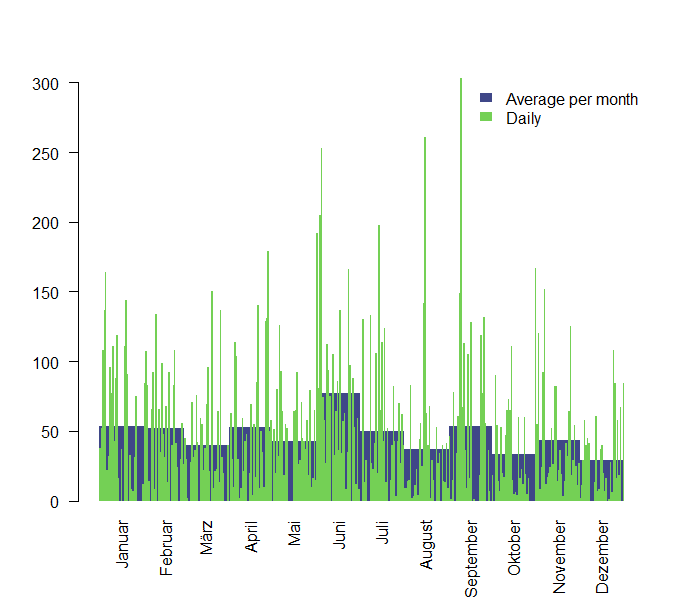
I listen to music mostly on my way to work on the bike between 7 and 8 am and between 5 and 6 pm. My most important statistic though is which time of the year I spent listening to music. I’m most interested in some specific days and an average play/month, that can tell me in which mood I was in. Therefore I created the function daily_month_plot . It plots the average plays per month and the daily plays in one plot. The average plays per month are visualized behind the daily spikes. Here you can see that February was a really quiet month for me.
data$daily_month_plot()
For some simple statistics, I also included an aggregation plotting function called barplots . It can plot aggregations per weekday, week, month or day. The data for this function is provided by the function bar_data .
data$barplots("weekdays")
weekly (starting with week 52 of 2017):
data$barplots(“week”)
Where I can clearly see that I was not really listening to a lot of music during the beginning of the year and my listening activity increased dramatically by week 18.
This post is a bit out of my spectrum, which mostly deals with packages about R packages being useful for Pharma. But I really like music and think music and data science make a good combination. Sound’s great together!
How would I miss to program just a little bit during the holiday season? But I didn’t want to work on something serious, so I decided to checkout some ground work on R-Shiny + JQuery + CSS. The result are some nice holiday greetings inside a shiny app:
I just googled CSS + holidays and what I found was this article on CSS for the holidays. The Pixel Art Christmas Tree I found from dodozhang21 really amazed me. But it was missing some shiny features. So I thought why not make it a custom shiny output? I was already writing about custom shiny inputs but never on custom shiny outputs.
Actually, the tree is kind of easy. I found that 83 rows of the CSS file account for the moving pixels of the tree as CSS keyframes. There are 5 keyframes (0% , 25%, 50%, 75%, 100% of the animation). So I read them as data.frames in R. Then I sampled X colors for the number of balls the user wants to find in the tree and replaced X of the 83 rows in 5 data frames. Then I put everything back into HTML by:
A few month ago I joined the R/Pharma conference in Cambridge, MA.
As a take away I thought of my project and how I can improve, with solutions others provided. Mainly solutions in R are R-packages. So I’m a R-Shiny programmer in a regulated environment, so the list of the solutions I took are mainly helping you, if you are providing a) Shiny Apps b) Statistical packages c) verified solutions. Let’s go and see which R-packages I did not know and now find really useful:
Packrat
What most of my co-workers are producing, are reports. Actually tons of statistical reports. As we work in a regulated environment, all reports are double-checked. Meaning you program it, and someone else programs it, too. You do not want to waste time, because there was an update of a mathematical package which leads to differences in a number. There is a really nice solution for that.
Packrat allows you to store all packages you are using for a certain session/project. The main guide for packrat can be found at the RStudio blog describing it.
Packrat will not only store all packages, but also all project files. It’s integrated in RStudio’s user interface. It allows you to share projects along different co-workers really fast.
The main lack I see is the need for a server, where you store all these packages. This should be solved with RStudio’s new Package Manager. Another disadvantage is the incompatibility with some packages. I noticed that I could not use the BH package under R-3.4.2 with packrat and had to find a work-around for that.
Diffdf
I have to tell you that I wasted nearly 30% of some of my days comparing data.frames. It’s an important task in testing statistical outcome or any calculations done with a statistical application you compiled. In Pharmaceutical and diagnostics applications one of the most relevant aspects is the validity of data. To ensure that the data we use in clinical studies, quality assurance or on a daily basis just getting data from a co-worker. For me this task has not only been hard, but even harder to document.
The diffdf package by Kieran Martin really solved that task. It not only provides you with a neat interface, but also with well arranged outcomes.
The basic diffdf example looks like this:
library(diffdf)
iris2 <- iris
for (i in 1:3) iris2[i,i] <- i^2
iris2$new_var <- "hello"
class(iris2$Species) <- "some class"
diffdf(iris, iris2)
You can see that basically one column is newly introduced, three values are changed in 3 different numeric columns and the type of a column is changed. All these three changes are displayed in a separate output. Additionally also things that did not change are mentioned, with can be really helpful, in case you do not check for full equality of the data frames you are comparing.
Differences found between the objects!

A summary is given below.

There are columns in BASE and COMPARE with different classes !!
All rows are shown in table below

  ==================================
   VARIABLE  CLASS.BASE  CLASS.COMP
  ----------------------------------
   Species     factor    some class
  ----------------------------------

There are columns in COMPARE that are not in BASE !!
All rows are shown in table below

  =========
   COLUMNS
  ---------
   new_var
  ---------

Not all Values Compared Equal
All rows are shown in table below

  =================================
     Variable    No of Differences
  ---------------------------------
   Sepal.Length          1
   Sepal.Width           1
   Petal.Length          1
  ---------------------------------


All rows are shown in table below

  ============================================
     VARIABLE    ..ROWNUMBER..  BASE  COMPARE
  --------------------------------------------
   Sepal.Length        1        5.1      1
  --------------------------------------------


All rows are shown in table below

  ===========================================
    VARIABLE    ..ROWNUMBER..  BASE  COMPARE
  -------------------------------------------
   Sepal.Width        2         3       4
  -------------------------------------------


All rows are shown in table below

  ============================================
     VARIABLE    ..ROWNUMBER..  BASE  COMPARE
  --------------------------------------------
   Petal.Length        3        1.3      9
  --------------------------------------------
The output is easily readable and covers all the information you need to do the expected: comparing two data frames. What I really like is the quick feedback on how many differences were observed. In case you have a lot of differences, expect you added +1 to every value of a column, you can immediately see this in the summary.
Additionally the detailed information, given not only the value difference, but also the position of the value in the table, is a huge advantage. Sometimes analyzing large cohorts of patients, can reveal a difference in measurement 99,880 and you do not want to scroll through a table of “matches” until you find this one difference. Therefore this detail view is a huge advantage against other packages.
Archivist
An R package designed to improve the management of results of data analysis. Key functionalities of this package include:
(i) management of local and remote repositories which contain R objects and their meta-data (objects’ properties and relations between them);
(ii) archiving R objects to repositories;
(iii) sharing and retrieving objects (and it’s pedigree) by their unique hooks;
(iv) searching for objects with specific properties or relations to other objects;
(v) verification of object’s identity and context of it’s creation.
This can be really important in reproducible data analytics. In pharmacological projects you often have to reproduce cases after really long time. The archivist package allows to store models, data sets and whole R objects, which can also be functions or expressions, in files. Now you can store the file in a long-term data storage and even after 10 years, using packrat + archivist you’ll be able to reproduce your study.
Example for task (ii) — restore models
This example gives a list of models stored inside the package
A data.frame comes with in my repository at https://github.com/zappingseb/RPharma2018packages in the arepo folder. Your task is to create a new data.frame, store it in the arepo_new folder and add it to the restored data.frame. If everything works out the sum of the data.frames shows up to be 2 for position (1,1).
You can see in this task, that my old data.frame is not only stored as a data.frame, but also with a distinct and reproducible md5 hash. This makes it incredibly easy to find stuff in a few years again and showcase that it’s the exact piece you needed.
logR
The logR package can be used to basically log steps of your analysis. In case you have a lot of steps in your analysis and need to know, how long these take, what was the status (error, warning) and what was the exact call, you can use logR to store everything that was done. logR therefore connects to a PostGres database and logs all steps of your analysis there. I can highly recommend to use logR in case you’re not sure if your analysis will go through running it a second time. logR will check each one of your steps, therefore any failure is stored. If your next step runs just because of any environment variable, that was set, you can definitely see this. Here is the basic example for logR from the author:
library(logR)

# setup connection, default to env vars: `POSTGRES_DB`, etc.
# if you have docker then: docker run --rm -p 127.0.0.1:5432:5432 -e POSTGRES_PASSWORD=postgres --name pg-logr postgres:9.5
logR_connect()
# [1] TRUE

# create logr table
logR_schema()

# make some logging and calls

logR(1+2) # OK
#[1] 3
logR(log(-1)) # warning
#[1] NaN
f = function() stop("an error")
logR(r <- f()) # stop
#NULL
g = function(n) data.frame(a=sample(letters, n, TRUE))
logR(df <- g(4)) # out rows
#  a
#1 u
#2 c
#3 w
#4 p

# try CTRL+C / 'stop' button to interrupt
logR(Sys.sleep(15))

# wrapper to: dbReadTable(conn = getOption("logR.conn"), name = "logr")
logR_dump()
#   logr_id              logr_start          expr    status alert                logr_end      timing in_rows out_rows  mail message cond_call  cond_message
#1:       1 2016-02-08 16:35:00.148         1 + 2   success FALSE 2016-02-08 16:35:00.157 0.000049163      NA       NA FALSE      NA        NA            NA
#2:       2 2016-02-08 16:35:00.164       log(-1)   warning  TRUE 2016-02-08 16:35:00.171 0.000170801      NA       NA FALSE      NA   log(-1) NaNs produced
#3:       3 2016-02-08 16:35:00.180      r <- f()     error  TRUE 2016-02-08 16:35:00.187 0.000136896      NA       NA FALSE      NA       f()      an error
#4:       4 2016-02-08 16:35:00.197    df <- g(4)   success FALSE 2016-02-08 16:35:00.213 0.000696145      NA        4 FALSE      NA        NA            NA
#5:       5 2016-02-08 16:35:00.223 Sys.sleep(15) interrupt  TRUE 2016-02-08 16:35:05.434 5.202319000      NA       NA FALSE      NA        NA            NA
We often build up shiny apps that need local PC settings to perform well. For example did we build a shiny app that accesses a MySQL database by the Active Directory login of the user. To get the Active Directory Credentials without a login window, we just ran the shiny app locally. As not all users in the department knew how to run R + runApp() , RInno sounds like a great solution for me.
RInno packs your shiny app into an .exe file that your users can run directly on their PC. This would also allow them to use fancy ggplot functionalities on locally stored Excel files. This can be really important in case data is under security protection and cannot be uploaded to a server. The tutorial given by the developer can help you a lot to understand the issue and how to solve it.
A package containing all measures you might need to evaluate the predictive power of a statistical model. I came across this package in one of the first sessions. Whenever we think of a proper way how to measure the difference between our model and the data, we discussed a lot of different ways. Of course it’s simple to write sqrt(sum((x-y)**2)) but it looks way better in yardstick two_class_example %>% rmse(x, y) . In yardstick you know where your data is coming from and you can easily exchange the function rmse while in the example I’ve shown you need to re-code the whole functionality. Yardstick will save a lot of discussions in our team in the future. Happy it came out.
Wer sich schon immer einmal fragte, wie man einen mittelmäßig trainierten Radfahrer ordentlich fordern kann, hier kommt die Antwort. Im Spätherbst durch Frankreich fahren ist eine Idee. Ich nahm die wunderbare Route von Freiburg im Breisgau über Clermond-Ferrand nach Bordeaux auf mich. Es hat 5 von 7 Tagen geregnet, an den beiden Tagen an denen es nicht geregnet hat, war es dafür saukalt (unter 5°C). Wie man hier sehen wird gab es lecker Essen, schöne Landschaften und viele viele Kühe auf der Tour. Am Ende war das Wetter in Bordeaux sogar der Hit und neben Schmerzen in den Beinen habe ich auch noch viel über meine Grenzen gelernt.
Der erste Tag – 103,07 km – 4h28m – 552m
An Tag 1 will man ja nicht sofort aufgeben. Aber die ersten 50 km hat es bei starkem Wind geschüttet wie blöde und ich konnte nach 20 km schon einmal meine Handschuhe auswringen. Zum Glück hat es dann aufgehört und der Wind blies mich über die Ausläufer der Vogesen hinweg nach Belfort. Sehr sehenswert ist dort das Fort und die Wälder rund herum.
Freiburg – Ensisheim – Belfort
Der zweite Tag – 158,45km – 6h 59min – 1.495m
Südlich von Belfort erstreckt sich Wald mit hübschen kleinen Dörfern und viel nichts. Besancon ist dann eine deutliche Abwechslung, eine richtige Stadt. Im L’Annexe bekam ich leckeres Essen und super Tipps, wie ich den Rest der Route gestalten sollte. In Dole gibt’s außer einem sehr schönen Kanal-Hafen tatsächlich nichts.
Belfort – Villersexel – Besancon – Dole
Der dritte Tag – 104km – 6h 10min – 802m
Regen ist ja tatsächlich ganz ok, aber wenn es einem den mit 50 km/h ins Gesicht schlägt, dann hört der Spaß auf. Ich musste mehrfach umdrehen und entschied mich dann den Zug (TER) nach Chalons-sur-Saone zu nehmen. Ein nettes Städtchen, wo es im Le Bistrot sehr gutes Essen gab. Der Nachmittag führte über die Weinberge des Burgund und den Canal du Centre entlang bis nach Monteau-les-Mines von wo aus ich den Zug in das wunderschöne Paray-le-Monial nahm.
Dole – Saint-Jean-de-Losne – Nuits-Saint-George – TER
Chalons-sur-Saone – Jambles – Monteau-les-Mines – TER – Paray-le-Monial
Der vierte Tag – 135,26km – 7h 12min – 966m
Tag 4 war mit zwei Bergetappen und dem schönen Kurort Vichy angekündigt. Auf der ersten Bergetappe lag leider unglaublich viel Schnee und es regnete. Dazu hatte ich dann kurz vorm höchsten Punkt der Tour auch noch einen Platten. Kein guter Anfang. Zum Glück konnte das Essen im Le Caudalies mich wieder aufwärmen. So ging es noch einen Berg hinauf und dann mit fettem Gegenwind immer Richtung Clermond-Ferrand. Hier empfing mich Magalie mit einem köstlichen und großartigen Abendessen.
Feiertag in Frankreich und Deutschland war der 1.11. Deshalb waren alle anderen auf dem Friedhof und ich am Berg. 600 Höhenmeter hinauf zum Col-de-Ceyssat ging es erstmal noch direkt vor dem Frühstück. Oben angekommen steht man vor der wunderschönen Kulisse des Corez und kann sich die nächsten Stunden an weiteren 1000 Höhenmetern in dieser hügeligen Landschaft ohne Menschen und ohne Autos erfreuen. Ein bisschen geregnet hat’s dabei natürlich auch wieder. Im Dorf Peyrelevade gab es zum Glück eine geöffnete Unterkunft (Ante Mille), in der ich der einzige Gast war. Sogar der Dorfladen hatte am nächsten Morgen auf.
Clermond-Ferrand – Col-de-Ceyssat – Peyrelevade
Der sechste Tag – 154,11 km – 7h 1min – 1.486m
Meine Prämisse für diesen Tag, raus aus dem nichts. Das Corez galt es für mich noch zu durchqueren. Kein Restaurant hatte offen und so konnte ich mir neben schönen Berghängen mit Wäldern im Regen auch das Dörflein Segur-le-Chateau mit seinen schönen Fachwerkhäusern anschauen. Irgendwann hat man es heraus aus dem Wald geschafft und ist im Schlösserpark Perigord angekommen. Hier staunt man nicht schlecht über die vielen Chateaus und auch der Dom von Perigueux ist natürlich eine Augenweide.
Am nebligen Morgen ging es durch die wirklich saukalte Dordogne. Vorbei an weißen Kreidefelsen und wunderschönen Schlössern hoffte ich stundenlang auf die Sonne. Diese zeigte sich dann endlich in den Weinbergen der Cote de Bordeaux. Einen Abstecher ins schöne St Emilion konnte ich mir dort nicht verkneifen, allerdings ist auch Libourne sehr sehenswert. Noch ein paar Hügelchen ging es auf dem Weg nach Bordeaux zu überqueren, doch dann war ich finally fertig!
Software can save lifes! — R and Python programming language rank in the Top10 of programming languages today. Both languages come out of open-source and research environments and are now moving into the industry. Testing software is really essential in industry. Why to talk about human readable tests?
Let me introduce you to my working environment. On a daily basis I’m writing code in R. From this code we build software that is applied in projects every day. A lot of people agree on the fact that software shall be tested. Even deeply tested until 100% code coverage is reached. OK, if you do not agree, you can stop reading now.
Additionally my work influences people’s life, directly. Not only their life, but whether they stay alive. I’m writing code in a clinical environment. So a feature in my software that was not tested could mean my software produces an outcome, that your doctor interprets wrong which can cause you pain, because he takes a wrong treatment decision. So far so good, the same accounts for a guy who coded the micro controller software of your car’s steering wheel. If you steer left because you do not want to hit a wall, you do not want your car to steer right and leave you flat and dead. Such software shall be deeply tested, too.
The clinical environment and regulatory authorities
Now what’s special about software in a clinical environment is that each application, whether it is a medical device or a drug itself or even just the process how to produce that drug has to be checked. This checking process is guided by the government. If you are taking a drug or your blood gets analyzed by a medical device, you want authorities to make sure that it saves your life or at least makes you healthier. If you’re from the U.S., the authority is called FDA and will do that for you. In case you’re living in Europe, find out which of our 26 different authorities is responsible for you, in Germany it’s the TÜV, in France it’s the ANSM.
Let’s focus, I’ll limit the scope of these authorities a bit. I would like to talk about a classical example from clinical applications like a Urine test strip. Everybody has seen such a thing. They can test e.g. for sugar in your Urine. If there was sugar in your Urine, you should be checked for Diabetes. So, the authority has to make sure, that the whole process around the test strip improves your diagnosis. The authority makes sure the test strip can tell you if you shall be further analyzed for Diabetes. If you have Diabetes, the test strip shall at least give a hint.
Let’s make the scope a bit smaller. To evaluate the test strip after it was dipped into your Urine, a doctor plugs it into a test strip reader. The reader gives the result of your test as a number. How does it do that? There is a software evaluating the measurements of the sensor and printing the test outcome to a display due to a specific algorithm. Now regulatory authorities have to have the ability to check that:
the algorithm is right.
the algorithm was implemented right.
the software takes the right input from the right sensor.
the display of the device gets the right outcome of the software.
Step 1 basically needs good documentation of the software and the algorithm. This is a different topic. Step 2–4 can be done by software testing, in best case automated testing. Let’s assume sensor and display are working fine and are tested already.
The test case
The device I just made up shall be tested now. It consists of a sensor and a display and in between sits a chip that runs a software.
We now have to have a set of numbers that come from the sensor which result in a set of numbers that shall be displayed on the screen of the device:
Sensor Value    Display Value
3               12
5               15
5.5             15
8               24
1               too low to evaluate
3               12
2.9             12
24.2            too high to evaluate
Now the algorithm might not be clear to you. But guess there is a detailed description available:
The algorithm of device123 shall evaluate values smaller than 2 as “too low to be evaluated”, values smaller than 5 as “12”, values smaller than 7 as “15”, values smaller than 15 as “24” and values above 15 as “too high to be evaluated”.
The task of the regulatory authority is not to test the algorithm if they shall approve device123. There job is to check that the producer of the device checked the algorithm and its software implementation. Therefore the two following things have to exist:
Test cases
A test report telling how the test cases were evaluated
Test cases in the programming language R can be written with the packages Runitor testthat. Both allow developers and testers to check the software. The test cases shown above in the code box could look like this in testthate.g.
test_that("1 is interpreted correctly", {
  expect_equal(device123(sensor=1),"too low to evaluate")
})
test_that("8 is evaluated correctly", { expect_equal(device123(sensor=8),24)})
...
Now for people who read R code every day, this seems great. The testthatpackage will tell you if your function device123 upon being called with 1 or 8 gives the exact value. The only problem is, test_that does not tell you if your test was successful, what was your expected value, what was the input. This tiny tool will just tell you how many tests were run and which failed. See the reference from Hadley Wickham’s blog:
Each line represents a test file. Each . represents a passed test. Each number represents a failed test. The numbers index into a list of failures that provides more details:
1. Failure(@test-device123.R#5): 8 is interpreted correcty -----device123(8) not equal to 24Mean relative difference: 3
Now it assumes that all tests ran and you can check that those were successful. But the outcome is just command line stuff and just readable for people who are used to R.
I would like to come back to you as a patient. You pay the regulatory authority with your taxes. Do you expect the guy at the regulatory authority to know R or that cryptic stuff that comes out of it? Do you really expect walking into your doctors office and seeing a “proof” sign at his devices, which tells that someone at the authority looked into the code of this device?
My answer is no. I want the regulatory authority to be keen on the values the device gives to the doctor and maybe on the chemistry of the test strip, but software shall be something that works and does the described job. If it is well documented, it shall follow its documentation. Now the responsibility for the test cases lies at the side of the company writing the software. This company has to show the authority that the software was tested. The authority just has to make sure, this process was valid.
How do we allow regulatory authorities to understand test cases?
Now we know that automated software testing allows to check if device123 has the right algorithm implemented. The major problem we have is reading the code, test the code and check if the test was valid. Testing code with code seems not to be the right option to see if it’s valid. For a company it will be hard to tell the authority, see we tested code with code. We have a bunch of cryptic command line outputs you can read that proof it.
No, you want something nice.
In case you’re a .NET developer there is a really simple solution for this. It is called specflow. It generates really easy to interpret human readable test cases:
Feature: Device123. We prepare a device that can use our algorithm to get a screen value out of a sensor value.
Scenario: Check number 1
Given the sensor measures 1 in the device
Then the result should be "too low to evaluate" on the screen
Scenario: Check number 8
Given the sensor measures 8 in the device
Then the result should be 24 on the screen
The outcome of those tests is given in pretty reports:
But I’m not a .NET developer and making use of specflow to code tests in R or Python is rather hard.
A solution for human readable tests in R
In our team came up with a solution for human readable tests called RTest. It’s an R-package that allows to use XML files for testing other R-packages and gives reports in form of documents. We know that XML is not as nice as pseudo language, but as a beginning I think it’s a great way to start. Our XML files for the example would look like this:
<device.TestCase>
<ID>Test Case1</ID>
<synopsis>
    <author>Sebastian Wolf</author>
    <date>2018-05-25</date>
    <desc>Test device123</desc>
</synopsis>
<tests>
    <device test-desc="Test return value of input 1">
     <params><sensor value="1" type="numeric"/></params>
     <reference>
      <variable value="too low to evaluate" type="character"/>
     </reference>
    </device>
    <device test-desc="Test return value of input 8">
     <params><sensor value="8" type="numeric"/></params>
     <reference>
      <variable value="24" type="numeric"/>
     </reference>
    </device>
</tests>
</device.TestCase>
This setup not only allows to define numerical functions to test the algorithm inside the device but also to note some basic environment information, like who really wrote this test and when he started to write the test. This information shall of course be verified by the source-code control and a co-developer.
The outcome using RTest would look similar to this:
The test report not only shows for each test how it was executed but also the execution time, if it was successful, the reference value and the outcome. Someone who knows what the software shall do from the algorithm description can now by reading the test case and the test report, see what was tested and also see if this makes sense. For co-workers who are new to the project, it is also way easier to find into the project. Reading test cases and report outcomes allows them to see in a minute which parts of the project still have problems or which functions are not yet tested.
Summary
Understanding how R software was validated now does not need an R programmer anymore. The environment presented here allows people to see how the software was tested. I think that human-readable tests will make statistical software more fail-proof, easier to understand and more sophisticated. As R’s way out of a research environment into clinical environments or even car industries took place already, the process is not finished, yet. Many more tools will be needed to allow regulatory authorities to trust in such a big open-source project. Human readable test cases are a first step in helping companies to support the validity of their open-source solutions. Using R and a good testing framework will make people’s life safer, because you’ll have not only great statistical tools but great validated statistical tools.
The ideas and opinions expressed in this post are those of the author alone, and are not to be construed as representing the opinions of his employer or anyone else.
A step by step guide on how to include custom inputs into R Shiny. This guide is going through an example of a custom input build from jQuery. After the tutorial you will be able to: Build your own front-end elements in shiny AND receive their values in R.
Why a second guide on building custom shiny inputs?
For more than two years we are developing one of the largest Shiny apps in the world. It’s large in terms of interaction items and lines of code. I already explained this in one of my former blog entries on how to write such an app. I used some techniques in Advanced R to build it.
Our customers wanted a lot of different custom inputs inside our app. They see a website on the internet and want exactly the same inside our shiny app. “Can we get this feature into the app?”. Upon this question I start reading the tutorial about custom inputs from RStudio again and often again. Don’t understand me wrong, it’s a great tutorial. But people tell me, they are missing the key message. I am missing a clear definition of steps you have to follow, to get your input ready to work.
For me it is sometimes really hard to reproduce what I did for one custom input in another custom input. This is the main reason why I am now creating this tutorial. There are key elements in implementing custom inputs that you shall think about. Some of them you will already be keen on, so you can ignore one or the other paragraph. But the one’s you do not know about, please read them carefully. And whenever you are building a new input, make sure you checked the 7 steps I will explain below.
My example is pretty artificial, but there is a reason for that. I want to make it hard to get the value of the input and use jQuery, because it has a lot of really cool features and is already included in shiny . So let’s imagine you want to define two colors. One is your bar border color, the other is your bar fill color. Both shall be entered using a color picker. Upon being too close (e.g. red and dark red) there shall be a little note on this. I will do this using the Telephones by region App from the Shiny Gallery because it includes a barplot. But let’s start from scratch
1 Know how to find fancy and easy to implement inputs
The app shall get two inputs that allow you to choose colors. Such inputs are called color pickers. This tutorial will deal with jQuery inputs. JQuery is easy to learn and already included in shiny. So let’s start searching for inputs by googling the following: “colorpicker jquery” .These are my results:
Results for googling jQuery colorpicker
Let’s double check the first two. The ColorPicker — jQuery plugin looks like that from the code description (https://www.eyecon.ro/colorpicker):
You can already see a difference in documentation. While spectrum gives you the HTML element to use + the JavaScript code, ColorPicker leaves you with some pure JavaScript code. This is something you should be aware of. If you use the first one, you might have to find out what the HTML has to look like on your own.
Second of all you shall be aware that it might be hard to derive the value of the color picker. Later in this tutorial I will talk about the getValue function of R-Shiny custom elements. In this case it is actually kind of easy, as the inputs work as real input elements. input elements can be read in jQuery using
$('input').val()
So please try to always use custom inputs that can be designed as html <input> elements. Additionally if the input like for spectrum is just a basic <input type="text"> you can stick to shiny standard inputs in your code, meaning you can reuse something like the shiny function textinputas it also produces a <input type="text"> element, but covers additional features like a label.
So for reasons of simplicity and documentation I will use the spectrum.js color picker.
Takeaway #1: Search for jQuery based tools that provide HTML in their tutorials
2 Know some basic HTML and JS for the setup
This chapter is about the front-end setup of your custom input element. Therefore you need to know some basic HTML. First thing to know: what is a class and what is an ID. Please read this at the desired links on w3schools if you do not know the difference.
Your custom input shall have both. An ID to make it easy to use the spectrum.js, or any other JavaScript feature you will stumble upon. Most of such special input features use IDs. Additionally you shall use a class, to make it reproducible. You may want to have multiple of your custom input elements in your final shiny app. Therefore they shall all get one class to look the same or behave the same.
The element we want to build shall be a div element with a specific ID and two color pickers inside. From the spectrum.js website we know one color picker looks like this:
Of course you do not want to hard code the word “custom” here. Using the glue-package we can generate a pretty nice id parser. Additionally wrapping our two textInputs inside a div function and use glue to also parse the JavaScript code inside. Finally we get a function that will generate an input element including two text inputs where one is shiny made and one is custom made by HTML code (see below). Additionally the necessary JavaScript code for spectrum.js is parsed underneath the elements. We use the value preferredFormat: 'hex' as we like to get hex color values in R as a return.
#' Function to return a DoubleColorPicker input
#' @param id (\code{character}) A web element ID, shall not contain dashes or underscores or colon
#' @param col_border (\code{character}) A hex code for the border color default value
#' @param col_fill (\code{character}) A hex code for the fill color default value
#' @return An \code{shiny::div} element with two color pickers
#' @author Sebastian Wolf \email{sebastian@@engel-wolf.com}
DoubleColorPickerInput <- function(id="fancycolorpicker", col_border = "#f00", col_fill="#00f"){

  # Return a div element of class "doubleclorpicker"
  div(
    id=id,
    class="doublecolorpicker",

    # Include two shiny textInputs
    textInput(inputId=glue("{id}-input-border"),label="Border Color",value = col_border),
    tags$label("Fill Color"),
    HTML(glue("<input type='text' id='{id}-input-fill' value='{col_fill}'/>")),

    # Include the Javascript code given by the spectrum.js website
    HTML(
      glue(
        "<script>
          $('#{id}-input-border').spectrum({{
            color: '{col_border}',
            preferredFormat: 'hex'
          }});
          $('#{id}-input-fill').spectrum({{
            color: '{col_fill}',
            preferredFormat: 'hex'
          }});
          </script>"

      )
    )# HTML
  )#div

}
Placing the spectrum.js and spectrum.css files at the right place
Now inside your shiny app there are just two files missing. You can find both in the spectrum.js tutorial. You need to source the JS and CSS files. This is necessary for the app to work. Therefore you download spectrum.js from their website and place the “spectrum.js” and “spectrum.css” files in the “www” directory of your app (here “customshinyinput”).
Now you can source both files using the html sourcing procedures:
Now you can see that spectrum.js took over your shiny::textInput and made it a color picker input. This is not really a custom input. But you can already see it is a nice feature that you can have a simple text input that allows you to read colors.
Note: This is not a custom shiny input, as we do not receive the input values, yet. In the next chapter we will make it a real custom input.
Takeaway #2: Try to use Shiny Input Elements inside your custom elements.
Takeaway #3: Do not forget to source the JavaScript and CSS files of your custom element.
Takeaway #4: Put a div container around your element and give it a special class.
3 Know how to start with the JavaScript InputBinding file
The first step to make your input a real custom input is creating a JavaScript file as described in the tutorial by RStudio. It has to contain three main elements.
The creation of your custom InputBinding
The extension of your custom InputBinding
The registration of your custom InputBinding
#1 and #3 are easy to do. Just give it a name and use the two functions
// #1
var DoubleColorPickerBinding = new Shiny.InputBinding();
// #3
Shiny.inputBindings.register(DoubleColorPickerBinding);
The hard part comes for Part #2. Part #2 shall contain 5 functions
find
getValue
setValue
subscribe
unsubscribe
Let’s start with the find function. The find function allows you to call your custom input inside all other (2–5) functions by the el variable. This is pretty nice to work with, as you don’t have to find the element again and again and again. In our case we defined that each custom input shall have the HTML class doublecolorpicker . To find the element, we just use:
where scope is the website you are working on and find is a function that comes with jQuery and the . operator of CSS calls for classes. Do not mess up the two different find functions. One is defined inside your JavaScript file, the other one comes from jQuery. Now you’ve got it. You found your custom input element again and can work inside it. The whole JavaScript file you need to add to your app now looks like this, in future we call it DoubleColorPickerInput.js:
// DoubleColorPicker Input Binding
//
// Definition of a Shiny InputBinding extension to
// get the values of two color pickers.
//
// https://github.com/zappingseb/customshinyinput
// Author: Sebastian Wolf
// License: MIT
// -----------------------------------------------------
// Create a shiny input binding
// Each custom input needs to be a shiny input binding
// that is defined by the JavaScript class "Shiny" and
// using the method "InputBinding"
// The name can be chosen, here it is "DoubleColorPickerBinding"
var DoubleColorPickerBinding = new Shiny.InputBinding();
// Extend the binding with the functions seen here
$.extend(DoubleColorPickerBinding, {
// The scope defines how the element is described in HTML code
// The best way to find the scope
find: function(scope) {
    return $(scope).find(".doublecolorpicker");
},
getValue: function(el) {
// todo
},
setValue: function(el, value) {
// todo
},
subscribe: function(el, callback) {
// todo
},
unsubscribe: function(el) {
// todo
}
});
// Registering the shiny input
//
// The following function call is used to tell shiny that
// there now is a new Shiny.InputBinding that it shall
// deal with and that it's functionality can be found in
// the variable "DoubleColorPickerBinding"
Shiny.inputBindings.register(DoubleColorPickerBinding);
Takeaway #5: Use the jQuery.find() function to get your element into the Shiny.InputBinding.
4 Know what your getValue function looks like
Here comes the hard part. We now want to access the value of our custom input and hand it over to R. Therefore we need to work on the getValue function inside the JavaScript file. This function basically returns the values of your custom input element into your shiny input variable.
The example I constructed makes it a bit harder than what you would expect. In this case we do not want to include just the value of one input element, but two. Therefore the best way to handle two values between JavaScript and R is the json-Format. It allows you to send dictionaries as well as arrays. Here we would like to get an array with dictionaries that tells us something like this: border_color=red, fill_color=blue. In JSON this would look like this
It means you get an array of two objects that both have the attributes name and the attributes color. We can do this now inside our getValue function by using some basic jQuery Tools.
getValue: function(el) {
  // create an empty output array
  var output = []

  // go over each input element inside the
  // defined InputBinding and add the ID
  // and the value as a dictionary to the output
  $(el).find("input").each(function(inputitem){

    output.push({
        name:   $(this).attr("id"),
        value:  $(this).val()
    });
  });

  // return the output as JSON
  return(JSON.stringify(output))

}
The functions you need to know are each, attrand val . These three functions allow you to iterate over your inputs (each), to derive their ID (attr) and to derive their value (val).
In the R Code of DoubleColorPickerInput.Rwe encoded the IDs an a way that they represent border color or for the fill color. The IDs make a good name by this encoding.
In case you want a more difficult input you might have to look up how to get the value of an element. It can be different than basically using the val function or you need a different find call. For example using a textarea input you cannot find it using the $(el).find('input') statement. You will have to use $(el).find('textarea') and also append the value of this element to your output array.
To make the output array readable in R you have to return it as a JSON string. Inside JavaScript the JSON.stringify function will do it for you.
Takeaway #6: Derive input element Values by jQuery.val()
Takeaway #7: Use JSON arrays to derive multiple input values
5 Know what your subscribe function looks like
Now we have a custom input using two color pickers and we are able to derive the value of this input. Next we need shiny to also react upon changes of this input. This is what is called subscribe.
There are two ways how you can subscribe to an input. The first one will use no rate policy, meaning you send everything that changes immediately to R. The second one can use a rate policy, meaning you wait a certain time for inputs to change and then send the values. The second one is really important for text input fields. In case somebody types a word, you do not want shiny to react upon each letter the person types, but on the whole word. Therefore you will need a rate policy. The rate policy is explained in detail inside the RStudio tutorial.
Here we would like our app to change on any color change we have in our DoubleColorPicker. As each element inside our DoubleColorPicker is an input, we can basically check for changes of those. Therefore jQuery contains a function that is called change that notices any change of the value of an element or changes of classes, too. Other candidates in jQuery for such change recognition of changes are: keyup , keydown , keypress .
Our subscription to the color pickers will look like this:
subscribe: function(el, callback) {
    // the jQuery "change" function allows you
    // to notice any change to your input elements
   $(el).on('change.input', function(event) {
     callback(false);
       // When called with false, it will NOT use the rate policy,
	  // so changes will be sent immediately
   });
  }
change.input seems like an easy thing to check on. But you might have more difficult inputs inside your shiny custom input element. Therefore I would recommend to give each of your custom inputs an additional class OR find out what is the class of your shiny-input. I built a shiny input out of shiny selectInput functions. They all have the class selectized . So you can make a subscribe function like that:
$(el).on('change.selectized', function(event) {
callback(false);
});
Instead of selectized you can insert your own class that you assign to each of your single elements. Assigning an own class like doublecolorpickerItem will also allow you to derive the values easier because you do not care for the type of your input element. The code of your app would look really different then, but you could do it and I recommend it. In case of this app here, it is not possible as shiny::textInput does not allow to set a custom class.
// DoubleColorPicker Input Binding
//
// Definition of a Shiny InputBinding extension to
// get the values of two color pickers.
//
// https://github.com/zappingseb/customshinyinput
// Author: Sebastian Wolf
// License: MIT

// -----------------------------------------------------

// Create a shiny input binding
// Each custom input needs to be a shiny input binding
// that is defined by the JavaScript class "Shiny" and
// using the method "InputBinding"
// The name can be chosen, here it is "DoubleColorPickerBinding"
var DoubleColorPickerBinding = new Shiny.InputBinding();

// Extend the binding with the functions seen here
$.extend(DoubleColorPickerBinding, {

  // The scope defines how the element is described in HTML code
  // The best way to find the scope
  find: function(scope) {
    return $(scope).find(".doublecolorpicker");
  },
  getValue: function(el) {
    // create an empty output array
    var output = []

    // go over each input element inside the
    // defined InputBinding and add the ID
    // and the value as a dictionary to the output
    $(el).find("input").each(function(inputitem){

      output.push({
          name:   $(this).attr("id"),
          value:  $(this).val()
      });
    });

    // return the output as JSON
    return(JSON.stringify(output))

  },
  setValue: function(el, value) {
   // todo
  },
  subscribe: function(el, callback) {
    // the jQuery "change" function allows you
    // to notice any change to your input elements
  	$(el).on('change.input', function(event) {
  	  callback(false);
  	});
  },
  unsubscribe: function(el) {
    $(el).off('.doublecolorpicker');
  }
});

// Registering the shiny input
//
// The following function call is used to tell shiny that
// there now is a new Shiny.InputBinding that it shall
// deal with and that it's functionality can be found in
// the variable "DoubleColorPickerBinding"
Shiny.inputBindings.register(DoubleColorPickerBinding);
it also contains an unsubscribe function, which you can always do in the same way using the off function.
Takeaway #8: Use the jQuery.change() function to derive changes of inputs.
Takeaway #9: Try to give each element inside your custom input a desired HTML/CSS class.
6 Know how to handle the input
Now we have a custom input that allows you to read two color pickers into one JSON string. This JSON string is available inside R by a shiny input. Additionally changes on one of the two colors will do a callback to shiny and inform it, that it has to react. We are finished with our custom input? No, we want it to come out of the JavaScript interaction not as a JSON string, but as a nice and readable list like:
[["fill"]]
"#f00000"
[["border"]]
"#00000f"
Therefore we need to add a registerInputHandlerfunction call to our shiny application. This will allow you to not only have a custom input, but also a custom value derived from your custom input. It needs two things in the setup.
change the JavaScript file to allow it
add the function call before your server.R is source
1 The first step is easy. You basically have to change the JavaScript functions to contain the following:
2 The second part is just coding a function to get a list out of a JSON string in R. This can be done by jsonlite easily. jsonlite will return a data.frame that you can parse into a list. All of this has to happen inside the registerInputHandlerfunction call. You can add this code snippet to the file where you defined the custom input and it will be sourced upon starting the app.
# Try to remove the input Handler as shiny does not allow double input
# handlers
try({ removeInputHandler("DoubleColorPickerBinding") })

# Use the shiny registerInputHandler function to
# register a way to deal with the inputs coming
shiny::registerInputHandler(
  "DoubleColorPickerBinding",
  function(x, shinysession, name) {

    if(is.null(x)) {
      return(x)

    } else {
      # Parse return value from JSON into R format dataframe
      colors_df <- jsonlite::fromJSON(x)

      # Extract the values of the data frame as a list
      res <- list()

      res[["fill"]] <- colors_df$value[
        which(grepl(colors_df$name,pattern="fill"))
        ]
      res[["border"]] <- colors_df$value[
        which(grepl(colors_df$name,pattern="border"))
        ]

      return(res)
    }
  }
)
Takeaway #10: Use registerInputHandler function to parse the response from your custom input over into something useful in R.
7 Don’t build reactive stuff about you input in R, do as much as possible in JavaScript
Actually, you are done with the application. Get the shiny Telephones by Region example and make sure your ui.R sources DoubleColorPicker.R and contains DoubleColorPickerInput("myid") inside your sidePanel . Additionally your ui.R should have
At the beginning of this tutorial I told you about the one feature I want to have, that is easy to do in shiny, but you should not do it. It’s double checking if the two inserted colors are too close as e.g. red and dark red. This feature comes along with calculating something from your input, that does not change your R calls or R calculations, but your user interface. For example you want to give a warning upon the two colors being too close to each other. Of course you can do it in R, but this means the following:
Pick the color → check the value with the inputBinding → send it to shiny → use the inputHandler → run R code on it → change a shiny warning output
You can get this much faster using pure JavaScript
Pick the color → check the value → change a warning item
Of course the 5 step process via shiny runs fast and you wont’t notice any difficulties if you have one custom input, but upon having maybe 20 or 30 of those inputs, we noticed in our apps, that they get kind of slow. This could be due to our bad R code or our bad JavaScript code. But we have 5 places where we can do something wrong. The second way just has 3 places to do something wrong. Therefore whenever you want to do something simple with your custom input that does not influence R calculations, do it in JavaScript.
My solution for dealing with colors comparison came from a stackoverflow entry.
As the response we need a warning HTML item (class=’warning’) and a function call to check the item by its ID. Both can be setup in shiny. The warning shall not be shown at the beginning (display: none) and have red text (color:red). The function call shall check for changes of the item using the jQuery.change function.
HTML(glue("
  <script>
    $('#{id}').on('change',
       function(){{
         check_doublecolorpicker('{id}');
       }});
   </script>"
)),
HTML("
   <div class='warning'
     style='color:red;display:none'>
     Please choose more different colors
   </div>"
)
The function check_doublecolorpicker needs to be set up in JavaScript. You basically need a function that gets the two color values, calculates the closeness and changes a warning HTML item. For calculating the closeness hexColorDelta was found in the stackoverflow entry and the rest is using the jQuery.val function as we did before. The jQuery.hide and jQuery.show function allow you to change the display property of your warning item. You have to use .warning as it’s class is warning and the . operator of CSS allows you to access class elements.
// Function to check a doublecolorpicker
// item by id
function check_doublecolorpicker(id){

  // derive an empty array of two inputs with
  // colors
  values = [];

  // push the two colors into the array
  $("#"+id).find('input').each(function(item){

    values.push($(this).val());

  });

  // derive the closeness of the two colors
  // delete the # sign by substring(1)
  closeness = hexColorDelta(values[0].substring(1),values[1].substring(1));

  // If the colros are too close, show a warning inside the
  // id element
  if(closeness>0.8){
    $('#'+id + ' div.warning').show();
  }else{
    $('#'+id + ' div.warning').hide();
  }
}
I know if your programming a lot in R and especially in R-Shiny, this does not suite you. The code in JavaScript looks different from code in R. But as I explained before, it may save you time and troubles. The outcome message will now show up in your app as this and we are done. 🙂
Warning message upon inserting two equal colors
Takeaway #11: JavaScript can save you calculation steps in your user interface
Summary
In summary I have to say that my blog post shall be named “7 steps to get custom inputs in shiny as easy as possible”. It is not easy to insert a custom input element into R-Shiny. It seems nearly impossible if you do not understand any JavaScipt. This tutorial should allow you to go through building up a new R-Shiny input by 7 steps. If you follow the 7 steps and do not forget to check one, you will succeed in building up new user interface elements. Those new elements will allow your users to insert something into your app they never thought about. We enabled things like a drag&drop input, an input to rearrange a bunch of plots on a grid, fancier check boxes, on-off switches, anything you can imagine. You can read whole books on fancy inputs or check websites like https://bootsnipp.com/ or https://freefrontend.com.
The main reason for such custom inputs shall be your user requirements. Of course you can put them into your app just to learn some JavaScript, but I don’t know if your boss will like it. But whenever your customer comes to you and shows you a website and says: “Can we get this feature into the app?”, now you should be able to answer: “Yes we can!”
Takeaways
Search for jQuery based tools that provide HTML tutorials
Try to use Shiny Input Elements inside your custom elements.
Do not forget to source the JavaScript and CSS files of your custom element.
Put a div container around your element and give it a special class.
Use the jQuery.find() function to get your element into the Shiny.InputBinding.
Derive input element Values by jQuery.val()
Use JSON arrays to derive multiple input values
Use the jQuery.change() function to derive changes of inputs.
Try to give each element inside your custom input a desired HTML class.
Use registerInputHandler function to parse the response from your custom input over into something useful in R.
JavaScript can save you calculation steps in your user interface
Use Thor’s hammer to get data scientists ready to work faster than you ever thought.
Welcome to your new office! Let’s take a look into your computer with your supervisor next to you saying:
Here is our working folder. Click through it and you’ll find out what we are doing. There is a list of software tools you’ll need to work with. Please install them. In case of any questions, ask Jamie.
Does this sound familiar to you? So what is so special about this if you are talking to people who use R. Actually nothing. But the text might start like this:
Here is our working folder. Folder A contains some really useful scripts, we call them hammers. Folder B contains some packages we started, we call them scissors and you find some packages we started on our github, these are the saws. We also have a package server, better install stuff from there. You can choose the R-Version you want to work with, Jamie has the most recent one, ask him how he does it. It would be great if you could use RStudio and get some common packages in it, maybe Jamie has a list of his favorite packages. Your most important project is inside our github. So please look through the folder structure. In case of any question, come to me, ask Jamie or check the wiki.
Yeah cool. These guys have a wiki. At least I can look something up. OK, they have three different places for R-packages and nobody knows which environment to work with, but I can handle this. Let’s go to Jamie and start.
When I saw systems like that for the first time, it really drove me crazy. Today’s Biostatisticians, Data Scientists or Software developers cost you more than 150 USD/hour. So you basically waste minimum two days if your startup structure is bad. I mean the structure you heard about does not seem bad, but it is. Taking into account you’ll need 30 minutes to get Jamie’s R-environment, 3 hours to install it, 5–6 hours to look through package folders, 5 hours or more to read the wiki and 2 hours to get access to github and then you still miss some system dependencies, this costs your minimum 2,325 USD. For this amount you can get a better computer or have free coffee for the whole year. So what can you do against it?
A pre-set up IDE installation — saves 2 hours
A standard R environment — saves 3 hours
A list of tools + a nice tutorial on installation — saves 5–6 hours
A fixed and standardized folder structure OR standardized project names — saves your life
A collection of vignettes — saves at least 5 hours
IDE installation
The integrated development environment (IDE) is the place to work for the guys in your office. It contains the connection to the source-code control system, the code editor, the console to run code, basically everything. You do not want somebody to waste time on getting this set up. So please have an install script that
installs the IDE
installs the extensions needed for your source code control systems and all links to that
installs all system components to work with this IDE (you hopefully know from your older projects)
installs a list of bookmarks to your important folders
sets up everything in a pre-defined folder or at least the extension repository. You can use a folder like:
C:\company_tools\IDEs\ourIDE
This IDE installation script will set up everybody in your department with the same IDE being installed at the same place. So you won’t hear questions like “How do I access github?” and the new people won’t have to call you because it says “It’s not possible to access version control without the following system components: XXX, XXX, XXX”.
In case the IDE crashes on the first day of the co-worker, you know where to look for it. This allows you to check for missing plugins and missing links in the system PATH . You think this just saves you 5 minutes, but each of the requests I mentioned is taking 5 minutes. Three simple questions and 15 minutes and 75 USD (0.25 hours * 150 USD/hour * 2 people) are gone.
A standard R environment
People working with R know how hard it is to share code with a co-worker. They have different package versions installed, they have the R environment in a different folder on their HD, they may even have a different R-version. All these troubles will occur, if you do not use packrat or RstudioConnect or RCloudfor each of your projects. And these troubles will definitely occur, even if you do so. But shall this happen at the first day a co-worker starts? Of course not.
So please give them a pre-defined R-version with a bunch of packages being pre-installed. I recommend to have at least 50, maybe a 100 packages you use on a daily basis, installed. Decide for one R-version that every co-worker needs to have installed with ~100 packages. Have an install script that installs it in a pre-defined folder. Something like
C:\company_tools\R\R-Versions\R-3.4.0-company
Please store the whole install script and the packages to be installed pre-compiled on a company repository. The install process shall not take forever and not everything needs to be recompiled. All people in your office shall have at least the same OS which allows you to store everything pre-compiled. This makes the whole R installation a copy&paste process and by this really fast.
A list of tools + tutorial
In one or the other R developer team people might want you to have a bunch of tools installed. For example in my group we use:
Miktex
ImageMagick
Ghostscript
LibreOffice
Pandoc
Java>1.8
git
qpdf
So if it is clear that sooner or later your co-worker will need these tools, please provide the guy with an installation script that downloads the most recent version, or a version you defined, for each tool and installs it.
Sometimes people will need admin rights to install all of these. So instead of requesting them for each single installation, they request them once and install all the stuff you told them to have.
If an install script is not suitable for you, write an entry in your wiki or a package vignette. This will contain all the steps needed to get the tools ready to work.
A fixed and standardized folder structure OR standardized project names
In R there are a lot of different working styles when it comes to folders and projects. My two major observations or working styles were:
people working on github and having RStudio projects
people working on shared drives/TFS/SVN and having sub-folder structures
1 For the people who work with project names, it is important to find a project, even if it was started years ago. Additionally you do not want to cause conflicts with your co-workers, because two projects have the same name. Moreover a project shall not contain all of the code developed in your department. Maybe it needs just 50 lines of code. So please define the following:
What is the naming convention for your projects e.g. username_task_month_year
What is the general size of your project e.g. one R-package, one script file, one script file + one data folder
Who is allowed to work on one project
Where do you list all projects e.g. a wiki, a specific website, a ticket management system
and the most important part: WRITE IT DOWN and make it available to everybody. If you have decided on these 4 parts, write it down, make it a working policy and kick peoples asses if they do not follow the rules. Else you’ll end up in chaos.
It will really help the guy at the first day who knows he has to find one of Jamie’s projects that deals with Clustering, as it might be called:
jamie123_clustering_patient_data_january_2017
2 For people who like folders and folder structures, I guess it is a bit easier. You may want to have the ability to find things after years, too. If you want to standardize the development of R-packages, research projects, test collections and report projects, those shall each look the same. A guy who developed one R-package in your company should be able to look into a second one and understand it in minutes. So please define the following:
What shall be the name of a certain project folder e.g. typeOfProject_name_month
Which sub-folders are needed for an R-package e.g. a change log folder, a releases folder, a test folder, a README.md file
Do you need separate folders for running projects vs packages? Shall they be stored at different places?
Is there any kind of folders that need to be existing for the storage of extensions, plugins, libraries?
and the most important part: WRITE IT DOWN and make it available to everybody. If you have decided on these 4 parts, write it down, make it a working policy and kick peoples asses if they do not follow the rules. Else you’ll end up in chaos.
I’m sorry that I was repeating myself, but I really needed to make my point.
Your collection of vignettes
This is a bit R specific. But instead of writing Confluence or Wiki entries, I really like the idea of using vignettes + pkgdown. For any development projects wikis are a nice tool to look things up. But inside wikis your code does not run immediately. In case you are writing vignettes to show your co-worker how certain things have to be done, you can check yourself. The code you write to document your installation scripts, your standard R-environment or even your folder structure has to work. Each single line of code can be executed inside the vignette.
Additionally vignettes are well known for R developers and they know they can access them via vignette() . Moreover the pkgdownpackage allows you to put the whole information on a website. This makes it a wiki again.
I also recommend to write such vignettes about your standard way on “How to build a package”, “How to document a function call in R Code”, “How to generate a knitR report with the right design” …. If you do all this in a nice and comprehensive way your co-worker won’t talk to Jamie, he’ll read your wiki. Instead of two people working, you’ll just need one.
Of course the new guy should still have a coffee with Jamie to know what’s up 😉
Something left for pro’s
If you really want to make it easy for your co-workers, write an R-package that contains all this. It can contain the install scripts, the vignettes, functions for basic processes, a function that builds default folder structures, maybe even functions that start tickets for newbies at the global IT service desk. Put it all in a package and call it: thorshammer
This package will be the most important tool for the first hour of your co-worker!
I guess if you follow my instructions the whole setting up a co-worker process runs within an hour or maybe less. You could start the day like this.
Hey, welcome. This is your PC, please get admin rights, after please download the thorshammer package. It will be the one tool you need today. First run the welcome bash script. During the script runs you can read inside the wiki how it sets up your folder structure and the IDE and how you can work with our version control. We have some basic tutorials how we do things in thorshammer, so please use it and see how we nail things down. After you nailed down a few planks, please have a coffee with Jamie to tell you what’s up next.
Nur zufällig war ich gleichzeitig mit der JRBB in Berlin. Auf dem XJazz Festival haben die Mädels und Jungs einfach krass gerockt. Das Publikum in Berlin weiß echt zu feiern und es gab sogar eine Sprung Einlage. Lautstark wurde eine lange Zugabe verlangt und naja, es war einfach geil Wie sagte Roman: Ihr seid geil, genau wie wir!
Es gibt diese Bands, die kennt man ewig und wollte sie schon immer einmal sehen. Dazu zählt bei mir Django Django. Die Jungs haben eine wirklich großartige Light-Show. Leider war ihre warm-up Band eine cool-down Band, allerdings klanglich ganz gut. Man of Moon sind wirklich sauber anzuhören und der Drummer gibt dauerhaft vollgas.
Django Django selbst leben von ihren Hits und ihrem ersten Album. Ähnlich wie bei Future Islands klingt jeder Titel annähernd gleich. Trotzdem geht da Publikum total steil und feiert komplett mit. Stage diving und crows surfing waren angesagt. Also eine echt fette Show. Meine Meinung nach war das trotzdem ein eher so mittelmäßiges Konzert, kann man gesehen haben, muss man aber nicht
Was für ein Line-Up. Jazzrausch Big Band, Meute und Brand Brauer Fink. Das Big Harry Festival fuhr die ganz großen Namen der Elektro Jazz Scene alle auf einen Schlag auf. Die Stimmung wurde Stück für Stück gesteigert, tanzbarer, lauter.
Von 20 Uhr bis 4 Uhr ging es in der Muffathalle bei einem der größten ein-Abend Jazzfestivals so richtig steil. Es wurde eigentlich dauerhaft getanzt und getrunken. Besonders Meute schafften es um 2 Uhr morgens noch einmal das Niveau zu steigern und großartig die Halle zu beschallen.
The albums of the year 2017 ordered by my personal listening. Find them as Playlists on the bottom. This year the analysis was performed with my own R-package library. Check it on github as the ananlyzelastfm R Package
Jazzrausch Big Band – Prague Calling
1 | Jazzrausch Big Band – Prague Calling
The greatest band from Munich whom we’ve seen live like a thousand times made it to rank #1 this year. Their first studio album is a great mix of dance/techno and jazz. It has a smooth sound and I loved to have it in my car. Do not miss out on their second album (JRBB Bruckners Breakdown)
2 | Kermit Ruffins – 1533 St. Philip Street
2 | Kermit Ruffins – 1533 St. Philip Street
In New Orleans this guy owns his own bar and is one of the most famous trumpet players in that city. It’s typical New Orleans sound, a bit oldschool, but great as ever.
3 | St Paul and the Broken Bones – Sea of Noise
3 | St Paul and the Broken Bones – Sea of Noise
I’ve seen this band live at the Love Supreme Festival this year. Paul Janeway is one of the craziest singers that I’ve ever seen. Even from far back in the audience you could feel his vibes and what a great dancer he is, too. The whole album is made to be performed live and nowhere else.
4 | Galactic – Crazyhorse Mongoose
4 | Galactic – Crazyhorse Mongoose
This album of Galactic was covered a few times. But I love the original funky fancy sound. A great album to have a funky relaxation.
5 | The Bamboos – The Best Of The Tru Thoughts Years
5 | The Bamboos – The Best Of The Tru Thoughts Years
This album is one of the best compositions I’ve listened to this year. The Bamboos have such a great variety of songs. Th music they play is between hip-hop, funk, soul and jazz. Together with other great artists at Tru Thoughs like Alice Russel, they made this the perfect album.
6 | Bilderbuch – Magic Life
6 | Bilderbuch – Magic Life
Why is the best German speaking band an Austrian band? Maybe Austria offers more time to think about how to make great, innovational music. The young guys of Bilderbuch offer a sound that was nearly never heard before. It has hip-hop choruses mixed with the guitar sound of the 70s. I think this is a masterpiece of German speaking music.
7 | Amy Winehouse – Back to Black
7 | Amy Winehouse – Back to Black
Again, again. I hope my kids will one day ask me, why this woman died so early. She’s just one of the greatest voices the world has ever seen.
8 | Miles Mosley – Uprising
8 | Miles Mosley – Uprising
Miles Mosley performed live at the Love Supreme Festival at three different gigs. This guy has a crazy variety in his baseplay. He can be a crazy guitar hero or a smooth jazz background play. You never know what will happen next on stage.
9 | Bonobo – Migrations
9 | Bonobo – Migrations
Whenever you get to a new Bonobo album, you think the last one was so great, it can never ever get better. And what happens? It gets better! This man is crazy. I don’t have any clue how he gets better from album to album, but he does it in great style.
10 | Electro Deluxe – Circle
10 | Electro Deluxe – Circle
The new album of Electro Deluxe is continuing the great tradition of dance albums. It has a strong and overall great sound.
11 | Hot 8 Brass Band – On the spot
12 | The Amazones – The Amazones
13 | Stanton Moore – Conversations
14 | Werkha – Colours of a red brick raft
15 | Jordan Rakei – Cloak
16 | Hot 8 Brass Band – Vicennial – 20 Years Of The Hot 8 Brass Band
17 | Trombone Shorty – Say that to say this
18 | Rebirth Brass Band – Ultimate Rebirth Brass band


_The_Amazons.jpg)
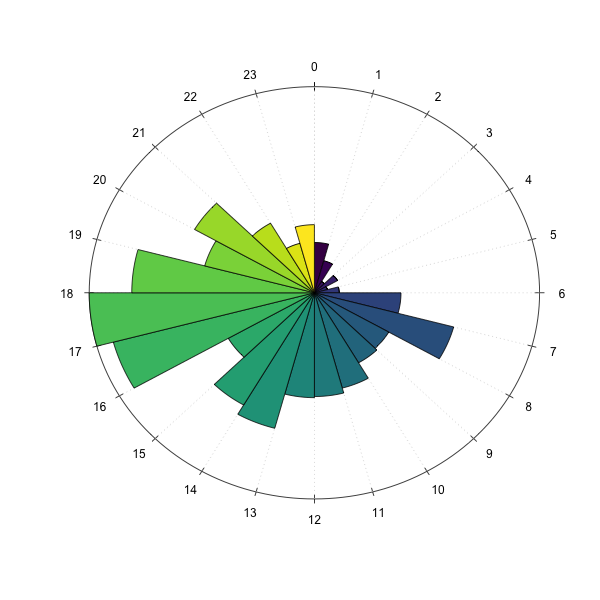
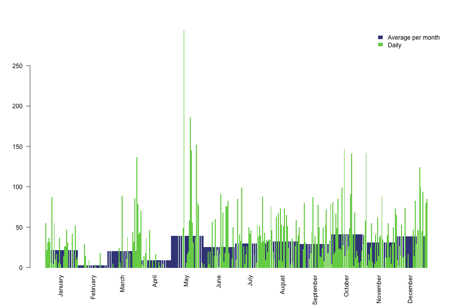

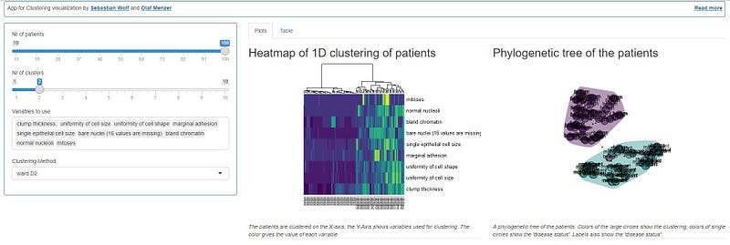

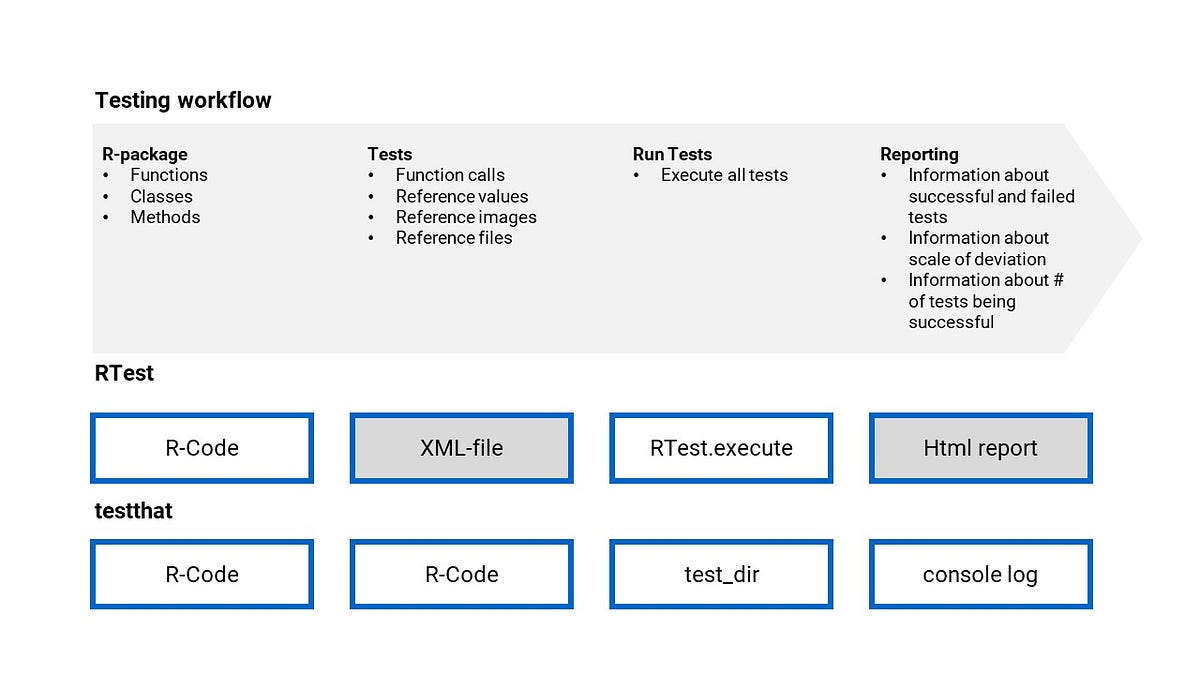
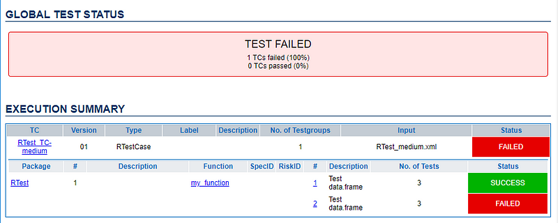
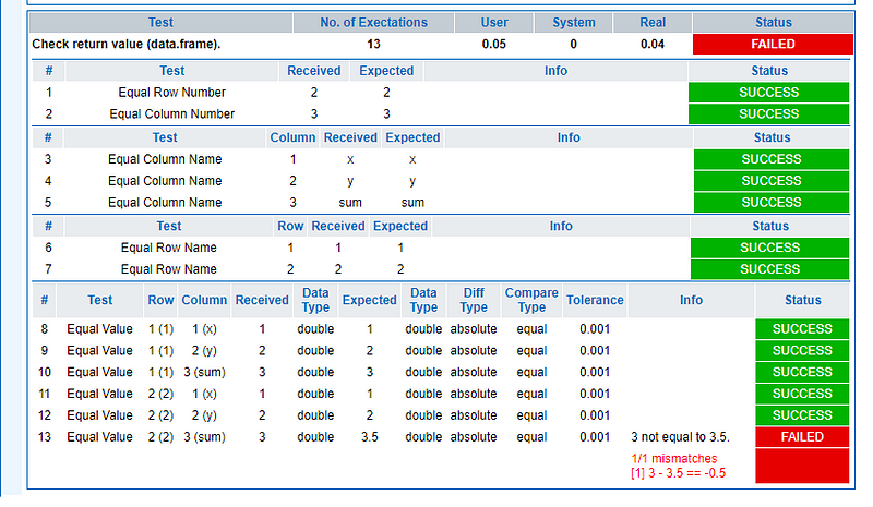

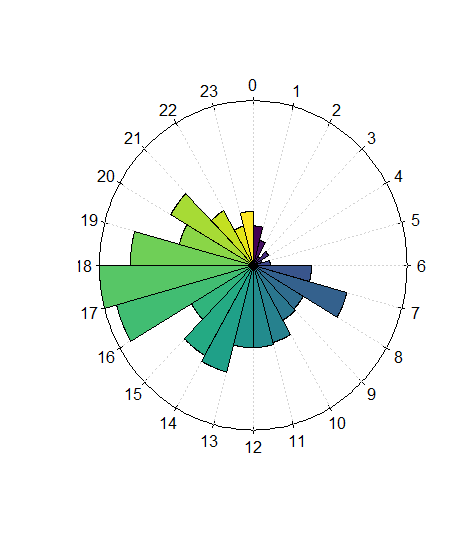
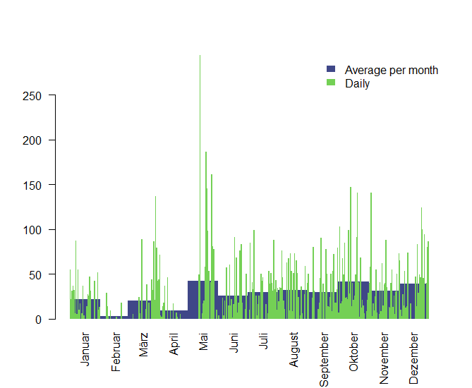
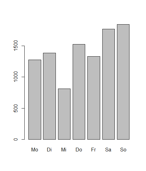
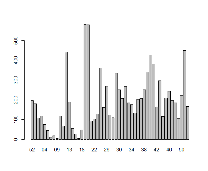


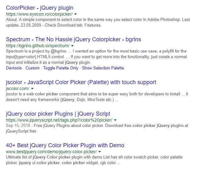
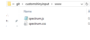
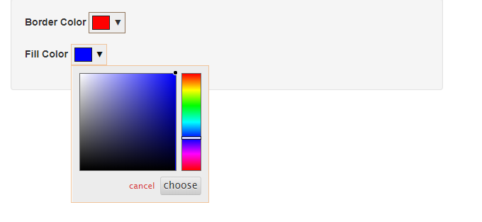
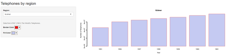
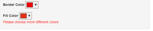


 11 | Hot 8 Brass Band – On the spot
 12 | The Amazones – The Amazones
 13 | Stanton Moore – Conversations
 14 | Werkha – Colours of a red brick raft
 15 | Jordan Rakei – Cloak
 16 | Hot 8 Brass Band – Vicennial – 20 Years Of The Hot 8 Brass Band
 17 | Trombone Shorty – Say that to say this
 18 | Rebirth Brass Band – Ultimate Rebirth Brass band
 19 | Clueso – Neuanfang
 20 | RAY BLK – DURT